Strain Gauge Principles and Strain Measurement

A loaded structure undergoes small deformations that may be difficult to see. A strain gauge is a common sensor for measuring how much a particular location stretches or contracts. In a tensile test, an extensometer measures the change in length between two reference points. A strain gauge instead converts deformation of a small grid bonded to the surface into an electrical signal.

An instrument may display strain as soon as the gauge is connected, but the output can increase or cancel depending on where the gauges are mounted and how they are wired. This article follows the measurement process from resistance changes in metal foil gauges—a type of electrical strain gauge—to strain data, then considers deformation in multiple directions and repeated loading over time.

1. Measuring Small Deformations Through Resistance Changes

Strain is the change in length divided by the original length. Taking tension as positive and compression as negative:

$$\varepsilon=\frac{\Delta L}{L_0}$$

If a 10 mm length increases by 0.01 mm, its strain is 0.001, or 0.1%. Small strains are commonly expressed in microstrain ($\mu\varepsilon$). Since $1\,\mu\varepsilon=10^{-6}$, this example corresponds to $1000\,\mu\varepsilon$. $1000\,\mu\varepsilon$ is not 1%; unit conversion matters. Strain is dimensionless because the numerator and denominator have the same units, although it is sometimes written as mm/mm to retain the length-ratio notation.

Construction of a Metal Foil Gauge

A metal foil strain gauge consists of a thin insulating backing carrying a narrow, elongated metallic grid. The figure below illustrates a typical product. Looking closely at the foil conductors reveals long runs concentrated in one direction and joined at their ends to form one long electrical path. These parallel runs define the primary measurement direction, so changing the mounting orientation can change the reading even at the same location on a structure.

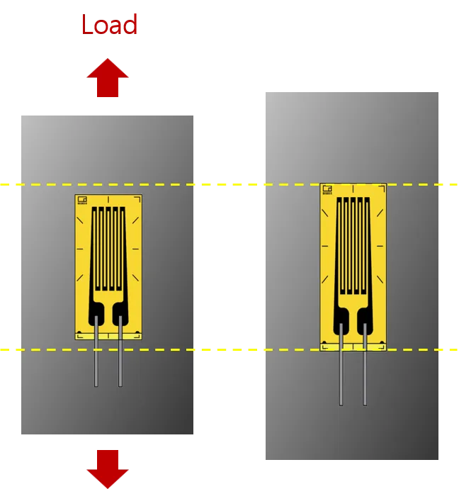
Typical metal foil grid geometry and its deformation as the specimen stretches. The left shows the initial state and the right the deformed state. Yellow dashed lines provide references for comparing the upper and lower gauge positions in the two states. Deformation is exaggerated for clarity.

Once the gauge is bonded to a specimen, surface deformation is transferred through the adhesive and backing to the grid. With ideal bonding and no slip or loss of strain transfer, the gauge and the specimen segment it covers extend or contract by the same amount. They therefore experience the same strain over that segment. The conductor length and cross-sectional area change, causing its electrical resistance to change. The gauge responds to deformation over the area occupied by its grid, rather than measuring an ideal mathematical point.

When illustrating gauge placement or orientation, a single elongated rectangle can represent a gauge without drawing every conductor. In this article’s simplified diagrams, the rectangle’s long axis represents the parallel grid direction and hence the measurement direction. The gauge-type illustration in Section 6 uses this convention.

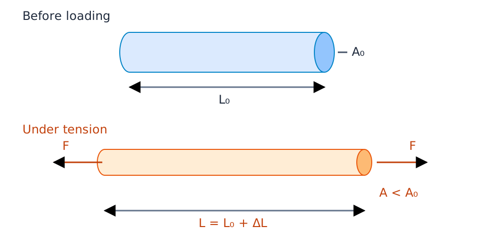
Axial tension lengthens a wire while reducing its cross-sectional area, measured perpendicular to the wire axis. Deformation is exaggerated for clarity. A metal foil gauge contains an arrangement of such conductive paths, whose resistance changes as the gauge deforms.

The resistance of a wire is:

$$R=\rho\frac{L}{A}$$

Here $\rho$ is resistivity, $L$ is wire length, and $A$ is cross-sectional area. Stretching a wire increases its length and reduces its area, so the resistance of a typical metal gauge increases. Compression reduces resistance. For small changes, expanding this expression gives:

$$\frac{\Delta R}{R}\approx\frac{\Delta\rho}{\rho}+\frac{\Delta L}{L}-\frac{\Delta A}{A}$$

For uniaxial deformation of the wire material with Poisson’s ratio $\nu_g$, $\Delta A/A\approx-2\nu_g\varepsilon$. Resistance changes therefore include changes in both geometry and resistivity. In practice these effects are combined into the gauge factor ($GF$).

Metal foil gauges are supplied with a gauge factor, typically around 2.1.

$$GF=\frac{\Delta R/R}{\varepsilon},\qquad \frac{\Delta R}{R}=GF\varepsilon$$

Metal foil gauges commonly have a $GF$ near 2, but calculations and DAQ settings should use the value supplied with the gauge. Distinguish the wire material’s $\nu_g$ from the test material’s Poisson’s ratio $\nu$. See NI’s strain measurement guide for background on foil gauges and gauge factor.

For $R=350\,\Omega$, $GF=2.0$, and $\varepsilon=1000\,\mu\varepsilon$:

$$\Delta R=350\times2.0\times0.001=0.7\,\Omega$$

The resistance changes from 350 Ω to 350.7 Ω. A Wheatstone bridge is commonly used to measure this small difference continuously.

Although the theory describes resistance changes, strain-measurement instruments can display strain directly, so you normally do not need to convert resistance readings yourself. When configuring the DAQ for a particular metal foil gauge, enter the nominal resistance specified for the purchased gauge.

2. What Does a Wheatstone Bridge Output?

The basic Wheatstone bridge configuration introduced here uses three fixed resistors and one variable resistor. The four resistors form a diamond, and the circuit measures the voltage difference between the two intermediate nodes. Whatever its drawing layout, it is electrically a comparison between two voltage dividers.

Three Fixed Resistors and One Variable Resistor

First, let resistor 1 be variable and resistors 2, 3, and 4 be fixed. Adjusting resistor 1 changes the left intermediate voltage, producing a difference relative to the right node. When all four resistances are equal, the intermediate voltages match and the output is zero.

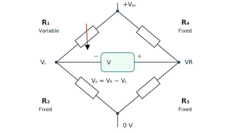
In this basic bridge, the arrow marks variable resistor R1; the other three are fixed. Arms run counterclockwise from the upper left, 1 → 2 → 3 → 4, with contribution signs + / − / + / −. Excitation is applied between the top and bottom nodes; the voltmeter reads the right node voltage minus the left.

Throughout this article, numbering runs counterclockwise from the upper left: 1→2→3→4. Thus 1 is upper left, 2 lower left, 3 lower right, and 4 upper right. With sequential numbering around the bridge, adjacent arms have opposite contribution signs and opposite arms have the same sign. Actual instrument terminal numbers may differ; check the wiring diagram.

Clockwise numbering is also possible. If you instead number across the bridge from left to right or right to left, the equations must be adjusted to match that assignment.

Define the output as $V_o=V_R-V_L$. With this numbering and polarity, the resistance-change and strain terms have signs $+,-,+,-$ in the order 1, 2, 3, 4. These are the coefficients describing each arm’s contribution, not an indication of whether a gauge is physically in tension or compression. Reversing the output leads reverses every sign, so numbering and output polarity must be defined together.

Let the excitation voltage between the top and bottom nodes be $V_{ex}$. Assuming the measuring instrument has sufficiently high input resistance to avoid appreciably loading the bridge:

$$V_L=V_{ex}\frac{R_2}{R_1+R_2},\qquad V_R=V_{ex}\frac{R_3}{R_3+R_4}$$ $$\frac{V_o}{V_{ex}}=\frac{R_3}{R_3+R_4}-\frac{R_2}{R_1+R_2}$$

Equal resistances give $V_L=V_R=V_{ex}/2$ and zero output. More generally, balance requires $R_1R_3=R_4R_2$. Adjusting the variable resistor disturbs that balance and produces a voltage difference.

For equal initial resistances $R$, write $R_i=R(1+\delta_i)$. The first-order approximation for small changes is shown below. Note the repeating +, −, +, − signs inside the parentheses.

$$\frac{V_o}{V_{ex}}\approx\frac{1}{4}(\delta_1-\delta_2+\delta_3-\delta_4)$$

Replacing the Variable Resistance with Strain Gauges

In a strain gauge, specimen deformation changes resistance instead of a manual adjustment. The following full-bridge example replaces all four resistors with gauges. Replacing only resistor 1 and retaining fixed resistors in arms 2, 3, and 4 produces a quarter bridge. The numbering and output polarity are identical in both diagrams.

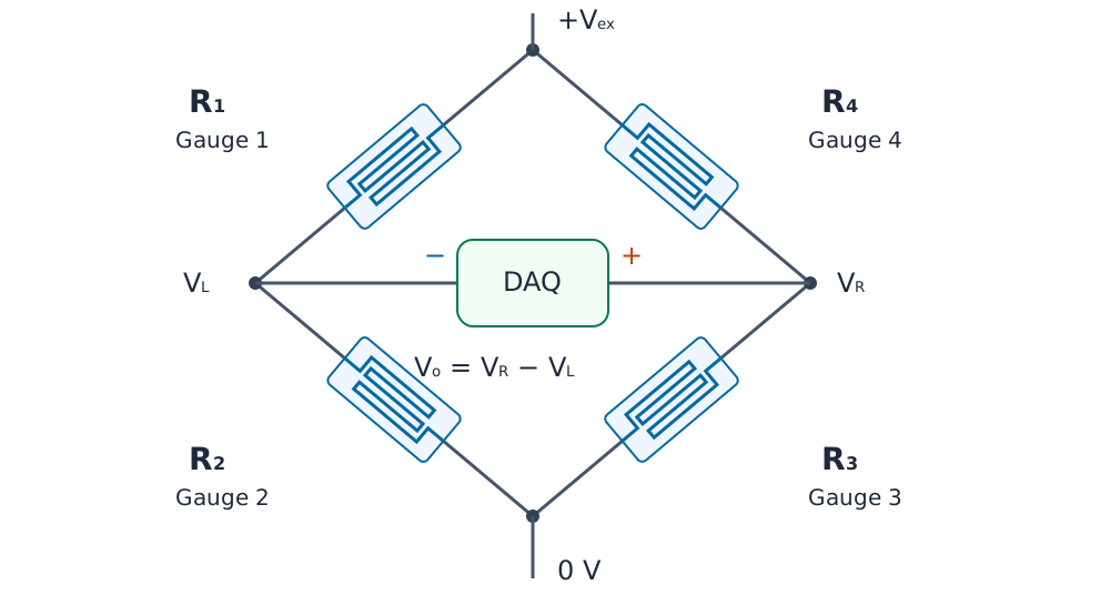
A full bridge with four strain gauges. Arms run counterclockwise from the upper left, 1 → 2 → 3 → 4, with contribution signs + / − / + / −. Grid symbols and numbers identify gauges and circuit arms, not mounting positions on the specimen.

For gauges with the same $GF$, neglecting temperature and wiring effects, the expression becomes the following. Set $\varepsilon_i=0$ for a fixed-resistor arm.

$$\boxed{\frac{V_o}{V_{ex}}\approx\frac{GF}{4}(\varepsilon_1-\varepsilon_2+\varepsilon_3-\varepsilon_4)}$$

Arms 1 and 3 have positive coefficients; arms 2 and 4 have negative coefficients. The same tensile strain can therefore contribute with either sign depending on the arm used. Reversing the DAQ signal leads reverses the overall output sign.

Quarter, Half, and Full Bridges

The examples below follow directly from this numbering. Here $\varepsilon$ is a positive strain magnitude. Bending examples assume equal and opposite strains on opposite surfaces.

Configuration	Gauge positions and strains	Remaining resistors	Approximate $V_o/V_{ex}$
Quarter bridge	Arm 1: $+\varepsilon$	Fixed resistors in 2, 3, 4	$GF\varepsilon/4$
Bending half bridge	Arm 1: $+\varepsilon$; arm 2: $-\varepsilon$	Fixed resistors in 3, 4	$GF\varepsilon/2$
Axial/transverse half bridge	Arm 1: $+\varepsilon$; arm 2: $-\nu\varepsilon$	Fixed resistors in 3, 4	$GF(1+\nu)\varepsilon/4$
Bending full bridge	Arms 1, 3: $+\varepsilon$; arms 2, 4: $-\varepsilon$	None	$GF\varepsilon$

The names quarter, half, and full bridge alone do not determine the strain conversion factor. The two half bridges above have different sensitivities: one measures bending on opposite faces, while the other combines axial extension and Poisson contraction under uniaxial stress. Select the DAQ’s specific bridge configuration to match the physical arrangement.

For a quarter bridge with only arm 1 changing, the exact expression is $V_o/V_{ex}=GF\varepsilon/(4+2GF\varepsilon)$. The table assumes $|GF\varepsilon|\ll1$. For larger strains, check whether the instrument applies nonlinearity correction.

3. Gauge-Position Quizzes

Does adding gauges always increase the output? Predict its sign and magnitude under these assumptions:

• All gauges have the same initial resistance and $GF$.
• Tensile and compressive surfaces have strains $+\varepsilon$ and $-\varepsilon$. All gauges run along the beam axis.
• Unused bridge arms contain fixed resistors of the same initial resistance.
• Temperature changes and lead resistance are ignored. Output is $V_R-V_L$.

The drawings show a beam bent by end moments M, with an exaggerated curved shape that puts the top in tension and the bottom in compression. Gauges follow the deformed surfaces. Short lines represent axial gauges; numbers identify bridge arms. Gauges on the same surface are assumed to experience equal strains.

Question 1. Gauge 1 on the Tensile Surface

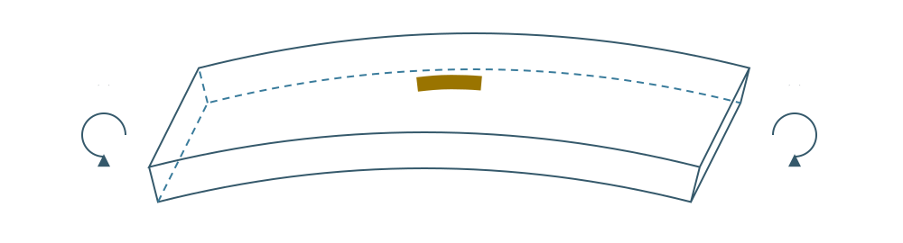
Question 1 gauge positions: gauges are arranged across each surface in this oblique view. Dark ochre gauges are on top; pale yellow gauges are on the bottom. Dashed lines show hidden bottom edges. G numbers identify bridge arms.

What is the reference output?

Question 2. Gauges 1 and 2 on the Same Tensile Surface

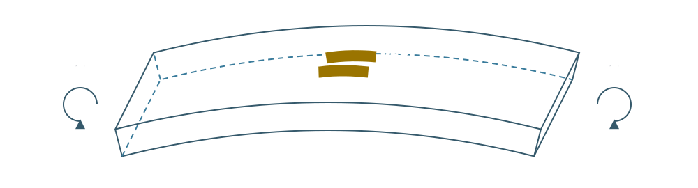
Question 2 gauge positions: gauges are arranged across each surface in this oblique view. Dark ochre gauges are on top; pale yellow gauges are on the bottom. Dashed lines show hidden bottom edges. G numbers identify bridge arms.

Do their contributions add?

Question 3. Gauges 1 and 3 on the Same Tensile Surface

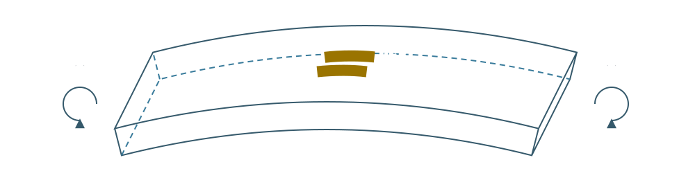
Question 3 gauge positions: gauges are arranged across each surface in this oblique view. Dark ochre gauges are on top; pale yellow gauges are on the bottom. Dashed lines show hidden bottom edges. G numbers identify bridge arms.

Is the result the same as in Question 2?

Question 4. Gauge 1 in Tension and Gauge 2 in Compression

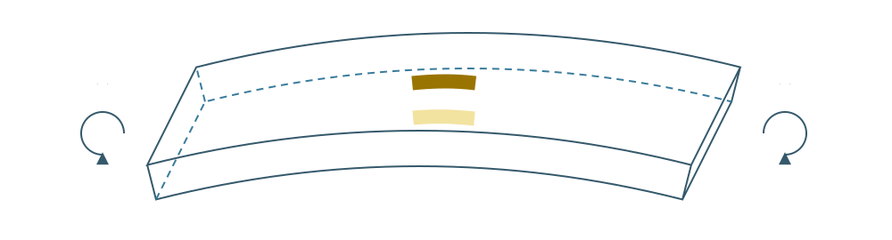
Question 4 gauge positions: gauges are arranged across each surface in this oblique view. Dark ochre gauges are on top; pale yellow gauges are on the bottom. Dashed lines show hidden bottom edges. G numbers identify bridge arms.

How does the compressive gauge contribute?

Question 5. Gauges 1 and 3 in Tension; Gauges 2 and 4 in Compression

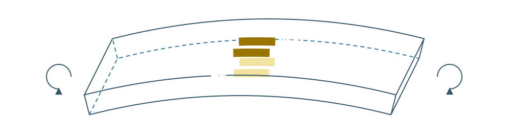
Question 5 gauge positions: gauges are arranged across each surface in this oblique view. Dark ochre gauges are on top; pale yellow gauges are on the bottom. Dashed lines show hidden bottom edges. G numbers identify bridge arms.

How does sensitivity compare with the quarter bridge?

Question 6. All Four Gauges on the Same Tensile Surface

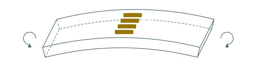
Question 6 gauge positions: gauges are arranged across each surface in this oblique view. Dark ochre gauges are on top; pale yellow gauges are on the bottom. Dashed lines show hidden bottom edges. G numbers identify bridge arms.

Does a full bridge always produce a large output?

Answers and Explanations

Define $q=GF\varepsilon/4$ and substitute the strains into $\varepsilon_1-\varepsilon_2+\varepsilon_3-\varepsilon_4$.

Question	Approximate $V_o/V_{ex}$	Explanation
1	$q$	Only the tensile strain in arm 1 contributes.
2	$0$	$\varepsilon-\varepsilon=0$: the contributions cancel.
3	$2q$	Arms 1 and 3 have the same coefficient sign, so their tensile contributions add.
4	$2q$	$\varepsilon-(-\varepsilon)=2\varepsilon$: the contributions add.
5	$4q$	All four terms contribute positively.
6	$0$	All resistances change by the same proportion, maintaining balance.

Under the ideal assumptions, Questions 2 and 6 give exactly zero even in the full voltage-divider equation. Real installations can retain an output because strains, gauge properties, or temperatures are not identical.

For $GF=2.0$, $\varepsilon=1000\,\mu\varepsilon$, and $V_{ex}=5$ V, Question 1 gives approximately 2.5 mV. Questions 3 and 4 give 5 mV, and Question 5 gives 10 mV. Zero output does not necessarily mean zero specimen deformation. First check whether the circuit adds the strain components you intend to measure.

Additional Quizzes: Can a Dummy Gauge Cancel Temperature Effects?

Questions 1–6 assumed constant temperature. Now consider changing ambient temperature. A dummy gauge is installed so that it experiences the same thermal response as the active gauge without receiving deformation from the test load. Here, an identical gauge is bonded under the same conditions to a separate specimen of the same material. The dummy experiences the same temperature change, without external loading or restraint of thermal expansion.

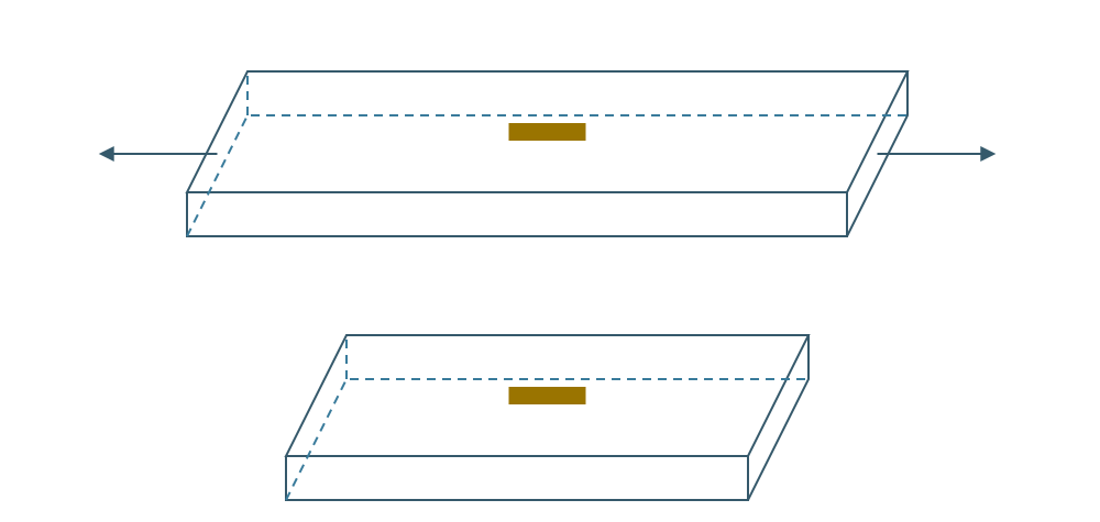
Temperature compensation with active and dummy gauges assumes the same temperature change, specimen material, gauge type, and bonding conditions. Gauge 1 responds to mechanical tension and temperature; the mechanically separate dummy responds to temperature without receiving the test bar’s load. Unloaded does not mean no free thermal expansion. Question 7 connects the dummy to R2, question 8 to R3, and question 9 asks what happens when the R2 dummy experiences a different temperature change.

Define the apparent strain caused by temperature as $\varepsilon_T$. A simple model for relative resistance change is:

$$\frac{\Delta R}{R}=GF(\varepsilon_m+\varepsilon_T)$$

Here $\varepsilon_T$ is the thermal resistance change divided by $GF$, not merely the material’s thermal expansion. The desired mechanical strain is $\varepsilon_m$. It equals $\varepsilon$ for active gauge 1 and zero for the dummy. Assume identical thermal responses and ideal, temperature-invariant fixed resistors in the other arms. Use a first-order approximation for small changes.

Question	Connection and conditions	What to predict
7	Active gauge in arm 1; dummy in arm 2	Does the thermal term cancel? Does mechanical sensitivity double?
8	Active gauge in arm 1; dummy in arm 3	Is equal temperature alone sufficient for compensation?
9	Question 7, but active and dummy thermal responses differ	What error remains?

Dummy-Gauge Answers and Explanations

The bridge coefficients are $+,-,+,-$. For Question 7, the thermal terms cancel:

$$\frac{V_o}{V_{ex}}\approx\frac{GF}{4}\big[(\varepsilon+\varepsilon_T)-\varepsilon_T\big] =\frac{GF\varepsilon}{4}$$

Only one gauge responds to the mechanical load, so mechanical sensitivity remains that of the quarter bridge. Using the bending half-bridge factor $GF\varepsilon/2$ would give an incorrect strain. Select the instrument setting for one active gauge and a compensation dummy, not simply for the number of physical gauges.

In Question 8, arms 1 and 3 have the same sign, so thermal contributions add:

$$\frac{V_o}{V_{ex}}\approx\frac{GF}{4}\big[(\varepsilon+\varepsilon_T)+\varepsilon_T\big] =\frac{GF}{4}(\varepsilon+2\varepsilon_T)$$

For Question 9, let the thermal responses be $\varepsilon_{T,a}$ and $\varepsilon_{T,d}$:

$$\frac{V_o}{V_{ex}}\approx\frac{GF}{4}\big[\varepsilon+(\varepsilon_{T,a}-\varepsilon_{T,d})\big]$$

Take $GF=2.0$, $V_{ex}=5$ V, and $\varepsilon=1000\,\mu\varepsilon$. For Questions 7 and 8, assume $\varepsilon_T=200\,\mu\varepsilon$ for both gauges. For Question 9, assume $200\,\mu\varepsilon$ for the active gauge and $100\,\mu\varepsilon$ for the dummy.

Question	Approximate output	Strain converted using the quarter-bridge factor
7	2.5 mV	$1000\,\mu\varepsilon$: thermal contribution canceled
8	3.5 mV	$1400\,\mu\varepsilon$: thermal contributions added
9	2.75 mV	$1100\,\mu\varepsilon$: residual error from the thermal-response difference

This compensation assumes matching thermal responses and small resistance changes. With temperature change alone and exactly matching relative resistance changes, Question 7 also retains zero output in the exact bridge equation. That does not eliminate every sensitivity change when mechanical loading is also present. Temperature gradients, thermal lag, bonding differences, and unequal self-heating can reduce compensation quality.

A fixed completion resistor is not equivalent to a temperature-compensating dummy gauge. Nor can a gauge simply rotated 90° on a loaded specimen be treated as mechanically unstrained: it measures Poisson contraction. See NI’s explanation of temperature effects.

4. From Gauge Installation to DAQ Measurement

A data acquisition system (DAQ) collects signals and stores digital data. Connecting two gauge wires to an ordinary voltage-input DAQ is not sufficient to measure strain. The system needs bridge completion resistors, excitation, and an amplifier and filters suitable for small differential voltages. Strain-input modules provide some or all of these functions.

A bridge box may be placed between the gauge and the instrument. It provides terminals and components such as precision bridge completion resistors. Supported gauge resistances and two- or three-wire connections vary by product. Distinguish it from a simple junction box. Excitation and amplification may or may not be included, so identify the functions performed by the box and the DAQ. An external box may be unnecessary if completion circuitry is already built into the DAQ module.

Surface deformation → adhesive and gauge → lead wires
                                              ↓
                  Completion circuit in bridge box or DAQ module
                                              ↓
                 Differential voltage → amplifier/filter → ADC → storage

Excitation supply ─────────────────→ bridge circuit

Choose Gauge Length for the Material and Measurement Objective

The important dimension is the active gauge length, rather than the overall backing size. A smaller gauge is not always better. The appropriate length depends on whether the goal is to measure a local stress concentration or the average deformation of a material containing multiple constituents.

Concrete is heterogeneous, consisting of aggregate and mortar. A short gauge placed over one aggregate may mainly read the relatively small deformation of that stiff particle, whereas a gauge over mortar or an interface may read differently. This can be a difference between the regions being measured, rather than simply sensor error.

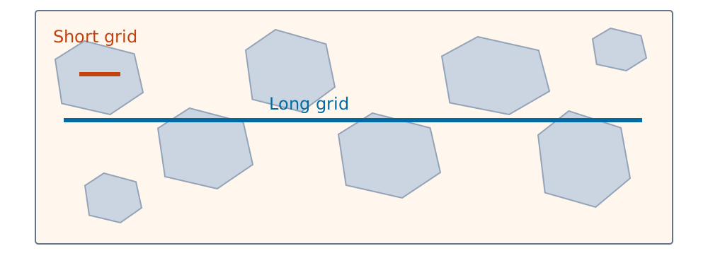
A short concrete gauge samples local strain; a long gauge averages across constituents. A short gauge on one aggregate may not represent the bulk concrete, so bulk measurements should span aggregates and mortar. Gray shapes are aggregates and the light background is mortar. This schematic specifies neither a particular mix nor recommended dimensions.

To obtain representative average strain in mass concrete containing large aggregates, such as that used in some dams, the measurement length must span enough aggregates and mortar. The aim is to average local variations, not simply discard small strains. Options include long surface-bonded gauges, long-gauge deformation sensors, and embedded sensors. Micro-Measurements’ concrete sensor overview discusses aggregate-related variation and the use of longer sensing lengths to average it.

Choose the length with the maximum aggregate size, mix, location, and purpose in mind; one gauge size cannot suit every dam. Conversely, a long gauge may smooth out the peak when the goal is to locate deformation near a crack. If it spans a crack, crack-opening displacement also contributes. Woven composites similarly require consideration of gauge length relative to the repeating fiber-bundle structure.

Bond Quality Determines Measurement Quality

First select the location and orientation for the measurement. Distinguish the tensile and compressive faces of a beam. For a stress concentration, ensure the grid is not too long relative to the region of interest. A long gauge averages a sharp local strain peak.

Follow the gauge and adhesive manufacturers’ procedures for surface preparation, cleaning, alignment, bonding, and curing. Poor strain transfer through the adhesive causes incorrect results even if the electrical circuit is sound. Secure cables separately so pulling forces do not reach the gauge or solder joints, and apply protection appropriate to the environment.

Composite Installation and ASTM D3039

ASTM D3039/D3039M covers in-plane tensile properties of polymer matrix composites. The following summarizes relevant provisions from Sections 7.3 and 11.6 of D3039/D3039M-08, whose text was available for review. It is not a verification of every requirement in the current edition. For a standards-based test, use the edition specified in the test plan. See ASTM’s edition listing and the 2008 text consulted.

• Location and orientation: place transducers symmetrically about the specimen’s mid-length and mid-width. Axial measurements on opposite faces allow bending to be evaluated for modulus determination. Poisson’s ratio requires axial and transverse measurements.
• Grid length: that edition recommends 6 mm for most materials and indicates that active lengths should not be below 3 mm. For woven laminates, consider a length at least as large as the weave repeat unit. This does not make 6 mm appropriate for every composite.
• Surface preparation: do not abrade through the matrix and expose or damage reinforcing fibers. Consult the gauge manufacturer’s composite-specific preparation and adhesive guidance.
• Heating and transverse sensitivity: select resistance and excitation to limit self-heating on materials with low thermal conductivity. Review transverse sensitivity, particularly for Poisson’s ratio measurements.

Practical preparation can proceed through location marking, compatible cleaning, minimal necessary abrasion, alignment, bonding and curing, cable restraint, and insulation checks. For conductive carbon-fiber composites, also check insulation between the surface and the gauge circuit. D3039 should not be treated as a universal installation manual specifying one adhesive and abrasive grade.

With matching axial gauges opposite each other on the front and rear faces, axial extension and small superimposed bending can be separated as:

$$\varepsilon_f=\varepsilon_{\mathrm{axial}}+\varepsilon_b,\qquad \varepsilon_r=\varepsilon_{\mathrm{axial}}-\varepsilon_b$$ $$\varepsilon_{\mathrm{axial}}=\frac{\varepsilon_f+\varepsilon_r}{2},\qquad \varepsilon_b=\frac{\varepsilon_f-\varepsilon_r}{2}$$

For front and rear readings of $1100\,\mu\varepsilon$ and $900\,\mu\varepsilon$, the average axial strain is $1000\,\mu\varepsilon$. Recording independent channels reveals both the average and the presence of bending. Connecting these gauges to arms 1 and 2 of the earlier bridge would cancel the common axial component, so keep the wiring consistent with the measurement objective.

A Quarter-Bridge Example

For the earlier 350 Ω gauge in arm 1, complete arms 2, 3, and 4 with appropriate precision resistors. Some may be internal to the module, while others may require an external adapter. For example, NI’s NI-9237 connection guide describes external quarter-bridge completion and wiring. Use the terminal diagram for the actual module.

How Two-, Three-, and Four-Wire Connections Affect Accuracy

The cable to a gauge has resistance too. Its influence increases with cable length and decreases with conductor cross-section, and it changes with temperature. Zeroing the initial offset does not automatically correct sensitivity loss or thermal drift during the test.

Connection	Treatment of lead resistance	Conditions to check
Two-wire single gauge	Both lead resistances are in series with the gauge.	Evaluate sensitivity changes from initial resistance and resistance changes during testing.
Three-wire quarter bridge	Corresponding leads enter different bridge arms so common changes cancel.	Lead resistances and temperature changes must match; check imbalance and residual sensitivity error.
Four-wire single-gauge measurement	Separate current and voltage-sensing paths, or a dedicated amplifier using sense leads to correct lead voltage drops.	The instrument must support the specific four-wire method and prescribed wiring.

The symmetry requirement for three-wire connections and an example of four-wire single-gauge wiring are given in the HBM MGCplus manual’s single-gauge connection section. Adding conductors to a two-wire input does not create a compensation function.

To estimate lead-wire error, consider the simple model of gauge resistance $R_g$ in series with the two lead resistances:

$$R_{\mathrm{meas}}=R_g+R_{L1}+R_{L2}$$

If a small change in lead resistance is interpreted entirely as gauge resistance change, its approximate equivalent strain error is:

$$\Delta\varepsilon_{\mathrm{lead}}\approx \frac{\Delta R_{L1}+\Delta R_{L2}}{GF\,R_g}$$

For $R_g=350\,\Omega$ and $GF=2.0$, a total lead-resistance change of 0.02 Ω corresponds to about $28.6\,\mu\varepsilon$. This illustrates the error scale when lead resistance is small relative to gauge resistance. Actual bridge correction depends on the instrument.

In a Kelvin four-wire resistance measurement, a known current $I$ flows through the current leads while separate sense leads, carrying almost no current, measure the gauge voltage $V_g$. Then $R_g=V_g/I$. Dedicated strain amplifiers implement four-wire circuits in different ways, so check their terminal diagrams. A four-wire full-bridge sensor cable usually contains two excitation and two output leads; it is not a Kelvin connection to a single gauge. A full bridge may use six wires to add remote excitation-voltage sensing. See HBK’s sensor cable explanation.

Practical Example: Bonding a 120 Ω Uniaxial Metal Foil Gauge and Wiring It with Three Leads

Consider a 120 Ω uniaxial gauge bonded to a flat metal surface and measured using a three-wire quarter bridge. The principle is the same as the 350 Ω example, but bridge completion and instrument settings must match 120 Ω. Composite surface preparation additionally requires the precautions against fiber damage described above.

1) Check the Product and Lead Configuration

Record the information on the package or data sheet before starting. Gauges that look similar may require different settings.

Item	What to check
Model and grid	Confirm a uniaxial pattern and suitable active length and measurement direction.
Nominal resistance	Confirm 120 Ω and assess measured resistance against product tolerance and lead resistance.
Gauge factor	Record the actual $GF$ from the package or certificate instead of assuming approximately 2.
Temperature conditions	Check thermal compensation for the specimen material, operating temperature, and strain limit.
Connection type	Identify solder pads, short leads, or preattached two-, three-, or four-conductor cable.
Bonding and measurement	Check the recommended adhesive and cure, excitation limits, and bridge-box support for 120 Ω and three-wire operation.

A short-lead gauge can be connected through a separate terminal bonded near the gauge and then extended with instrument cable. Do not let a long cable’s weight load the fine gauge leads. Connection options are described in HBK’s gauge selection guide.

To use a two-lead product in a three-wire circuit, prepare an approved connection with two wires at one gauge terminal and one at the other. A, B, and the wire numbers below are explanatory labels, not terminal names for a particular bridge box.

Gauge side                         Three-conductor cable to bridge box

 A o────────────────────────────── Wire 1
   │
 [120 Ω grid]
   │
 B o──────────┬─────────────────── Wire 2
              └─────────────────── Wire 3
              ↑
       Junction near the gauge

Wires 2 and 3 share the same electrical node at the gauge but connect to different instrument terminals as specified in its manual. Match the material, size, length, and temperature exposure of the corresponding leads to satisfy three-wire compensation conditions. Splitting a lead only at the bridge box while retaining a long two-wire cable does not compensate resistance changes in that original two-wire section. Any remaining short original leads also need to be considered. Rather than opening a sealed gauge assembly arbitrarily, choose an accessible connection design or a factory three-wire product. Micro-Measurements’ W3 option illustrates two electrically common contacts at one gauge node.

2) Degrease, Abrade, and Remove Debris

First remove oil and contamination with a cleaner compatible with the material. Abrading a dirty surface can embed contamination. Remove rust, paint, unstable oxide, and similar layers over an area larger than the gauge, then use the recommended abrasive to produce a uniform surface.

Some fine texture suitable for bonding is needed, but rougher is not always better. Deep grooves and large irregularities can produce uneven adhesive thickness. Abrasion direction affects the surface texture: follow the applicable instructions and change direction as appropriate for an even finish instead of producing deep scratches in one direction. A cross-hatched surface may be recommended for high-elongation installations. Do not apply one abrasive grade or roughness value to every material and adhesive. See Micro-Measurements’ surface preparation bulletin B-129.

Remove abrasive dust and residue using clean, lint-free wipes and a suitable cleaner. Use fresh wiping surfaces to carry contamination out rather than rubbing back and forth with a dirty wipe. Follow the specified sequence for systems requiring cleaning, conditioning, and neutralizing. Do not touch the cleaned surface or gauge bonding face; bond before recontamination occurs. KYOWA’s installation procedure also describes removing abrasive dust and wiping in one direction.

3) Align and Bond the Gauge

Mark the measurement axis and gauge center, then align the gauge’s index marks with these reference lines. Avoid deep scratches and remove marking residue during final cleaning. Angular alignment matters as well as position. A uniaxial gauge responds along its grid direction; if it is inclined to the intended axis, transverse and shear strain components affect the reading.

Use a dedicated strain-gauge adhesive suitable for the backing, specimen material, temperature, test duration, and strain range. Follow the prescribed quantity and working time to obtain a thin, uniform bond line. After positioning, avoid sliding or twisting the gauge.

For a room-temperature process that specifies finger pressure, place a clean PTFE (Teflon) sheet or other specified release film over the gauge and press through it. This prevents fingers from sticking to adhesive or contaminating the installation. The sheet goes above the gauge, not between it and the specimen. Some products specify polyethylene film or installation tape instead, so follow the supplied instructions. Distinguish the pressure-hold time from the full cure time. Do not substitute finger pressure for a process requiring heated or clamped curing. Examples of release films and curing methods appear in Micro-Measurements bulletin B-130 and KYOWA’s installation procedure.

4) Restrain the Leads and Connect the Bridge Box

After adequate curing, finish connections and soldering according to the product instructions. If a product requires wiring preparation before bonding, follow that sequence. Avoid excessive heat or tension at the joints. Leave a small amount of slack and restrain the cable separately so loads are not transferred to the gauge. Apply the necessary electrical insulation and moisture protection.

Follow the bridge-box manual’s diagram for a 120 Ω single gauge in a three-wire quarter bridge. Do not infer connections solely from wire colors or another product’s terminal numbers. Check the destinations of wires 2 and 3 from the common B node, and avoid duplicating completion circuitry between the box and the DAQ. Turn off excitation while making connections.

Before applying excitation, check for opens and shorts, terminal-to-terminal resistance, and insulation from the specimen. Use a resistance-test current suitable for the gauge and connected equipment, and follow the manufacturer’s limits for insulation-test voltage. Then enter the actual $GF$, 120 Ω resistance, and three-wire quarter-bridge configuration, and check zero and shunt response as described below. Do not simply reuse the excitation voltage from the 350 Ω example. At the same excitation in a balanced bridge, a lower-resistance gauge dissipates more heat. Select excitation for the 120 Ω product’s limits and the specimen’s ability to dissipate heat.

Configuration and Verification Sequence

1. Select the bridge type. Match quarter, half, or full bridge and the particular axial or bending arrangement.
2. Enter gauge data. Specify nominal resistance, $GF$, and specimen Poisson’s ratio where required.
3. Set excitation and input range. Consider output level, gauge self-heating, and instrument limits. The earlier 5 V is an example, not a recommendation for every gauge.
4. Set sampling and filters. Choose the required frequency band for static, impact, or vibration measurements.
5. Allow the unloaded signal to stabilize and zero it. Zeroing under load makes subsequent readings changes relative to that loaded state.
6. Perform shunt calibration. Connect a known resistor across the designated bridge arm and check the expected electrical response. This does not verify bond quality or mounting direction.
7. Apply a small test load. Check output sign and magnitude, and verify return to zero after unloading.

For a quarter bridge with only arm 1 active, a zero-corrected output of $V_o=2.5$ mV with $V_{ex}=5$ V and $GF=2.0$ gives:

$$\varepsilon\approx\frac{4}{GF}\frac{V_o}{V_{ex}} =\frac{4}{2.0}\frac{0.0025}{5}=0.001=1000\,\mu\varepsilon$$

The same voltage requires different conversion factors for half and full bridges. If the instrument already outputs strain, do not apply the factor a second time. Record clearly whether stored values are V, mV/V, dimensionless strain, or $\mu\varepsilon$.

5. Applications in Tensile and Cantilever Tests

Which Is More Accurate: an Extensometer or a Strain Gauge?

Both measure specimen deformation directly during tensile testing, but their measurement regions and error sources differ. An extensometer measures extension between two defined points, while a bonded gauge responds over its small grid area. Before comparing accuracy, check that the two measurements represent the same deformation state and comparable regions.

Aspect	Extensometer	Bonded strain gauge
Measurement region	Average strain between two reference points	Local average strain over the grid
Main error sources	Displacement calibration, gauge length, contact slip and mounting effects, optical tracking errors	$GF$, alignment, adhesive, temperature, transverse sensitivity, wiring, and DAQ
Small elastic strains	Check verified accuracy class and resolution over the range of interest	Suited to small signals, but bond quality and the entire measurement chain require verification
Large strains and fracture	Check travel, tracking, and removal requirements	Check grid and adhesive strain limits, debonding, and electrical failure

An extensometer’s calibration and classification apply over the relevant measurement range. Instron’s extensometer overview discusses gauge length, range, and calibration class as selection factors. Similarly, a gauge’s $GF$ accuracy alone does not describe the accuracy of the complete measurement.

For example, suppose an extensometer with a 50 mm gauge length has an extension error of 1 μm. Ignoring gauge-length error, its strain error is $0.001/50=20\,\mu\varepsilon$. Conversely, if true strain is $1000\,\mu\varepsilon$ but the entered $GF$ is 1% above its actual value, the calculated gauge strain is approximately $990.1\,\mu\varepsilon$. These assumed examples illustrate individual error sources; they are not a comparison of particular instruments.

The methods should agree well in a uniform elastic region, but bending or local damage can cause different readings. Before deciding that either sensor is wrong, compare measurement locations and lengths, front/rear strain, synchronization with load, and zero references.

Measuring Poisson’s Ratio from Axial and Transverse Strain

In a tensile test, Poisson’s ratio is obtained from transverse contraction relative to axial extension within the elastic region. Install axial and transverse gauges in a uniform central region, or use a 0°/90° biaxial rosette. Read the directions simultaneously on independent channels. Axial and transverse extensometers can also be used together.

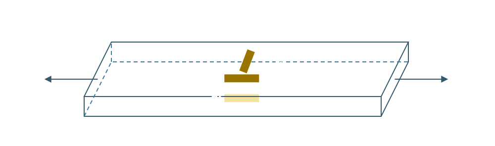
Oblique view of gauges for Poisson’s ratio and front/rear strain in a tensile test. Thick solid lines show the front axial and transverse gauges in dark ochre and the opposing rear axial gauge in pale yellow. εL and εT denote longitudinal and transverse strain. Align opposing axial grids to assess bending and read each grid on a separate channel. Place the transverse grid in a nearby uniform region, or use a biaxial rosette. This is not a standard specimen drawing.

1. Align the load axis and gauges, and use consistent zero and time references for both directions.
2. Select the start and end of the elastic strain interval required by the test method. Distinguish regions where damage or nonlinear behavior begins.
3. Determine axial change $\Delta\varepsilon_x$ and transverse change $\Delta\varepsilon_y$ between the same two times.
4. Calculate the interval Poisson’s ratio and record the interval and corrections used:

$$\nu_{xy}=-\frac{\Delta\varepsilon_y}{\Delta\varepsilon_x}$$

If axial strain increases from 1000 to $3000\,\mu\varepsilon$ while transverse strain changes from −300 to $-900\,\mu\varepsilon$:

$$\nu_{xy}=-\frac{-900-(-300)}{3000-1000}=0.30$$

Dividing instantaneous readings near zero strain can greatly amplify small zero errors. Use changes over an interval or, where the applicable method permits, the slope of $\varepsilon_y$ versus $\varepsilon_x$ within that interval. The interval above is an example, not a universal range for all materials.

Transverse strain may be smaller than axial strain, making alignment and transverse gauge sensitivity particularly important. Combining the two gauges into a single half-bridge output also makes their individual strains difficult to recover independently. For composites, record the loading direction and material axes; in general, $\nu_{xy}$ and $\nu_{yx}$ are not interchangeable.

Comparing Cantilever Surface Stress with Beam Theory

Consider a cantilever of length $L$, fixed at the left end and loaded downward by $P$ at the right free end. Its rectangular cross-section has width $b$ and thickness $h$. An axial gauge is bonded to the upper surface at distance $x_g$ from the free end toward the clamp. Here $x_g$ is the distance from the tip load to the gauge center; the distance from the clamp to the gauge center is $L-x_g$. For this loading direction, the upper surface is in tension and the lower surface in compression.

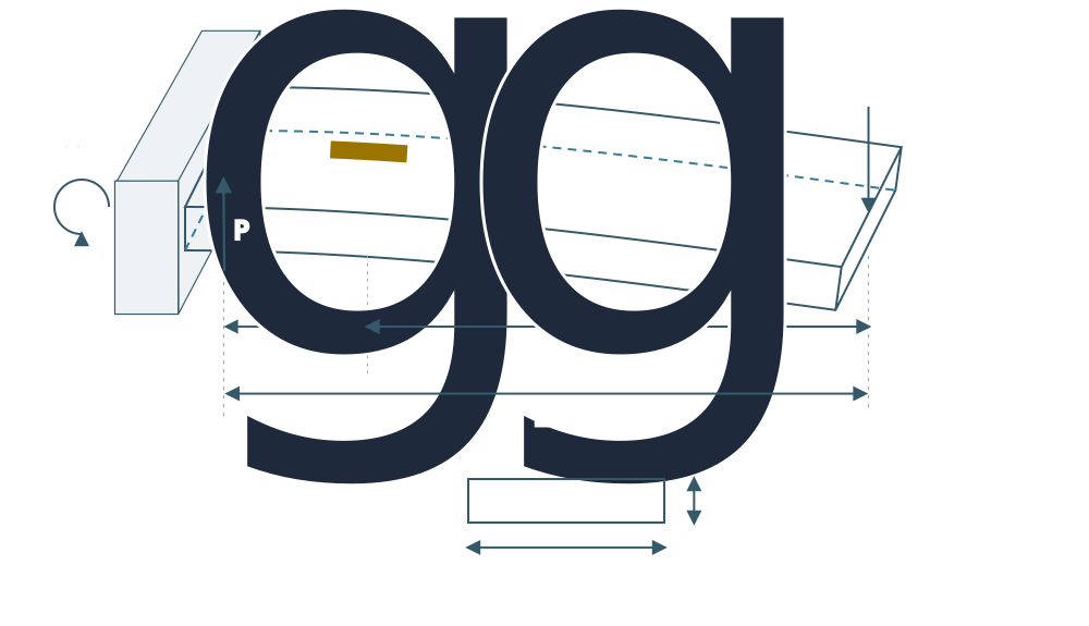
For a cantilever fixed at the left with a downward tip load, upper-surface strain gives the local stress. The distance $x_g$ from the gauge center to the free end determines the local bending moment; compare stresses at the gauge center. Deflection is exaggerated, with the gauge following the upper surface. M₀ = PL is the clamp reaction moment; dimensions $L$ and $x_g$ refer to the undeformed geometry.

Assume a homogeneous, isotropic, linearly elastic beam with small deflection and constant cross-section, neglecting self-weight. The bending-moment magnitude at the gauge and the second moment of area are:

$$|M(x_g)|=Px_g,\qquad I=\frac{bh^3}{12}$$

The upper surface lies $h/2$ from the neutral axis, so its theoretical tensile stress is:

$$\sigma_{\mathrm{theory}}(x_g)=\frac{|M(x_g)|(h/2)}{I} =\frac{6Px_g}{bh^2}$$

Experimentally, convert the measured axial surface strain $\varepsilon_g$, corrected for temperature, zero, and wiring effects, into stress. Where uniaxial stress is a reasonable approximation at the free surface:

$$\sigma_{\mathrm{exp}}=E\varepsilon_g$$

Take $E=200$ GPa, $L=300$ mm, $b=20$ mm, $h=5$ mm, $x_g=250$ mm, and $P=10$ N. The gauge center is therefore $L-x_g=50$ mm from the clamp:

$$I=\frac{20\times5^3}{12}=208.33\ \mathrm{mm^4},\qquad |M(x_g)|=10\times250=2500\ \mathrm{N\,mm}$$ $$\sigma_{\mathrm{theory}}=\frac{2500\times2.5}{208.33}=30.0\ \mathrm{MPa},\qquad \varepsilon_{\mathrm{theory}}=\frac{30.0}{200000}=150\,\mu\varepsilon$$

Now suppose the DAQ reads $147\,\mu\varepsilon$. The following uses assumed example data, not results from an actual experiment.

Quantity	Calculation	Result
Theoretical stress from load and dimensions	$6Px_g/(bh^2)$	30.0 MPa
Stress converted from the assumed strain reading	$200000\times147\times10^{-6}$	29.4 MPa
Relative difference from theory	$(29.4-30.0)/30.0\times100$	−2.0%

With the earlier quarter bridge, arm 1 active, $GF=2.0$, and $V_{ex}=5$ V, $147\,\mu\varepsilon$ gives approximately 0.3675 mV. If the reading has the opposite sign, first check loading direction, the instrumented face, and DAQ polarity.

Compare against stress at the gauge location, not the maximum clamp stress $6PL/(bh^2)$. For a sufficiently long uniform beam under only a tip load, bending moment varies linearly along its length, so a short gauge’s average can be compared with the value at its grid center. Separately consider local stresses near the clamp and load introduction, large deflection, thickness error, poor bonding, and differences in actual elastic modulus. The −2% difference in this example is not automatically the gauge’s own accuracy.

6. Rosette Gauges for Multiple Directions

Strain gauges are available with one, two, three, or more measurement directions. A one-axis gauge is also called a single-element or linear gauge. If the principal loading direction is unknown or stresses act in multiple directions, use a rosette containing closely positioned grids at different angles.

From left: a single-element gauge, two separate gauges placed perpendicular to each other, a biaxial rosette shown with overlapping elements, and a rectangular three-element rosette. Each yellow rectangle represents one grid, with its long axis indicating the measurement direction. Taking either diagonal as the reference, the three directions on the right correspond to 0°/45°/90°. This is a schematic, not a drawing of actual backing outlines or grid spacing.

Type	Typical grid directions	Application
Single-element / linear gauge	One direction	Measure strain along the selected direction
Biaxial / tee rosette	0°/90°	Compare axial and transverse strain; measure along known principal axes
Two-element shear / torque gauge	+45°/−45° to the shaft axis	Measure torsional shear strain and torque
Rectangular / 45° three-element rosette	0°/45°/90°	Calculate in-plane strain components and principal directions
Delta / 60° three-element rosette	0°/60°/120°	Recover the in-plane strain state from three directions

Three axes here means three directions on the surface, not direct measurement of every three-dimensional strain component, including through-thickness strain. To recover each directional strain separately, read each grid on an independent channel. Combining three grids into one bridge output does not retain enough information to recover the three individual strains.

Rosettes can have adjacent or stacked grids. In a strong strain gradient, differences in grid position affect the result. See Micro-Measurements TN-515 for selection and data-reduction details.

Two-Element ±45° Gauges for Torque Measurement

A shear/torque gauge combines two grids at +45° and −45° to the shaft axis on one backing; the grids are 90° apart. Under pure torsion of a circular shaft, they sense equal tensile and compressive normal strains. Their difference gives the shear strain.

Connecting the grids to adjacent half-bridge arms adds their resistance-change contributions, producing a differential torque signal rather than separate directional readings. A second pair on the opposite side can complete a four-grid full bridge. Convert the signal to torque using shaft geometry and shear modulus, or calibration with known torque. See Micro-Measurements’ shear and torque gauge guide.

Principal Strains from 0°/45°/90° Measurements

The following uses the in-plane transformation for small strains. Assume all grids represent the same local strain state, with 0° along $x$ and 90° along $y$. Strain in direction $\theta$, measured counterclockwise from $x$, is:

$$\varepsilon_\theta=\varepsilon_x\cos^2\theta+\varepsilon_y\sin^2\theta +\frac{\gamma_{xy}}{2}\sin2\theta$$

Here $\gamma_{xy}$ is engineering shear strain. With readings $\varepsilon_0$, $\varepsilon_{45}$, and $\varepsilon_{90}$:

$$\varepsilon_x=\varepsilon_0,\qquad \varepsilon_y=\varepsilon_{90},\qquad \gamma_{xy}=2\varepsilon_{45}-\varepsilon_0-\varepsilon_{90}$$

The eigenvalues of the symmetric strain tensor give the maximum and minimum in-plane principal strains:

$$\varepsilon_{1,2}=\frac{\varepsilon_x+\varepsilon_y}{2} \pm\sqrt{\left(\frac{\varepsilon_x-\varepsilon_y}{2}\right)^2 +\left(\frac{\gamma_{xy}}{2}\right)^2}$$

The direction of maximum principal strain is:

$$\theta_1=\frac{1}{2}\operatorname{atan2}(\gamma_{xy},\varepsilon_x-\varepsilon_y)$$

Using $\operatorname{atan2}(y,x)$ preserves quadrant information. The minimum principal direction is 90° away. When the principal strains are equal, the direction is not uniquely defined. Check the software’s argument order and angle units.

Converting Principal Strains to Principal Stresses

Measured strain does not determine stress without a material constitutive relation and assumptions about the stress state. Here assume an isotropic, linearly elastic material under plane stress, with negligible surface-normal and out-of-plane shear stresses. If temperature changes occur, separate free thermal expansion before calculating stress.

Under these conditions, principal stress and strain directions coincide, and the in-plane principal stresses are:

$$\sigma_1=\frac{E}{1-\nu^2}(\varepsilon_1+\nu\varepsilon_2),\qquad \sigma_2=\frac{E}{1-\nu^2}(\varepsilon_2+\nu\varepsilon_1)$$

For example, suppose the rosette readings are:

$$\varepsilon_0=600\,\mu\varepsilon,\quad \varepsilon_{45}=400\,\mu\varepsilon,\quad \varepsilon_{90}=-200\,\mu\varepsilon$$

Then $\gamma_{xy}=400\,\mu\varepsilon$, giving:

Quantity	Calculated value
Maximum in-plane principal strain $\varepsilon_1$	Approximately $647.2\,\mu\varepsilon$
Minimum in-plane principal strain $\varepsilon_2$	Approximately $-247.2\,\mu\varepsilon$
Maximum principal strain direction $\theta_1$	Approximately 13.3° counterclockwise from the 0° grid
$\sigma_1$ for $E=200$ GPa and $\nu=0.30$	Approximately 125.9 MPa
$\sigma_2$ under the same conditions	Approximately −11.7 MPa

Enter $647.2\,\mu\varepsilon$ as $647.2\times10^{-6}$ in stress calculations. These are in-plane results. Through-thickness strain is generally nonzero even under plane stress, so the in-plane principal strains should not automatically be called the maximum and minimum in three dimensions. The isotropic equations also cannot be applied directly to materials with directional properties, such as fiber-reinforced composites.

Measuring Residual Stress by Drilling at the Rosette Center

Rosettes can also help determine residual stress already present in a material. Welding, heat treatment, and forming can leave internal stresses after external loads are removed. Bonding and zeroing a gauge in that state alone does not reveal the existing stress, because the gauge measures subsequent deformation relative to its reference state.

The hole-drilling strain-gage method uses a dedicated three-element residual-stress rosette with space for a central hole. A precision drilling device is aligned with the rosette’s center mark and makes a small hole. This partially releases the surrounding stress. The resulting strain changes in three directions are measured and used to infer the stresses present before drilling. Use a dedicated rosette with a defined relationship between the hole and surrounding grids, rather than drilling arbitrarily through the grid of an ordinary rosette. See Micro-Measurements’ explanation of hole drilling.

The measurement sequence is:

1. Prepare the surface and bond the dedicated rosette without materially altering the existing residual-stress state during preparation.
2. Connect all three grids to independent channels. Record the pre-drilling reference after signal and temperature stabilization.
3. Align the tool with the center and drill incrementally to the specified depth without damaging the grids. Record relieved strains after drilling effects have stabilized at each step.
4. Calculate in-plane residual stresses and principal directions using hole diameter and depth, rosette geometry, elastic modulus, Poisson’s ratio, and calibration coefficients for those conditions.

The measured quantities are strain changes caused by stress relief during drilling. They cannot be inserted directly into the preceding ordinary-rosette stress equations, nor can $E\varepsilon$ simply be interpreted as the original residual stress. The inverse calculation must account for the stress field altered by the hole. Depth profiling also considers the influence of previous drilling increments; each increment’s strain change is not directly the stress in just that depth layer.

ASTM E837 addresses near-surface in-plane residual stresses in isotropic, linearly elastic materials. It uses shallow blind holes. Sensitivity decreases with depth, so it cannot reveal all stresses deep inside a component. Do not directly apply its standard interpretation where stress varies greatly across the hole diameter or to strongly anisotropic composites. See the ASTM E837 scope.

Because a hole remains, this is a semi-destructive method. Centering error, actual hole shape, drilling heat and induced deformation, and local plasticity can affect the result. Residual stress also affects fatigue behavior under later repeated loading. When interpreting it together with service strain histories, consider the measurement location and depth and the possibility of residual-stress relaxation.

7. Advanced Topic: From Strain Histories to Fatigue Analysis

Static testing often focuses on strain at a particular load. Real structures also experience acceleration, stopping, vibration, impact, and other repeated loads. The basic gauge data is a strain time history $\varepsilon(t)$. Converting it to stress histories and cycle counts provides input for fatigue assessment. The overall workflow is outlined in HBK’s explanation of the path from strain to lifetime.

Acquire Data That Can Be Analyzed Later

Choose a sample rate sufficiently above the highest frequency of interest and apply suitable anti-alias filtering before digitization. Barely satisfying the Nyquist criterion may not reproduce short impact peaks with the required accuracy. Check the bandwidth of the entire chain, including sensor, amplifier, filters, and sampling.

Channel synchronization matters when combining rosettes or gauges at different locations. Combining readings taken at different times can produce a strain state that never actually existed.

Store more than time and strain: include photographs of gauge locations and orientations, channel numbers, bridge configurations, $GF$, excitation, zero references, sampling rate, filter settings, temperature, and operating conditions. Preserve raw data and keep processed data separately with its processing settings. Automatically removing the mean can discard mean-stress information needed for fatigue assessment.

Rainflow Counting and Cumulative Damage

Under uniaxial linear elasticity, mechanical strain history can be converted using $\sigma(t)=E\varepsilon(t)$. For multiaxial loading, first calculate stress-component histories using the appropriate constitutive relation. A simple $E\varepsilon$ conversion is insufficient when plastic deformation is present.

Irregular stress histories contain cycles of different sizes. Rainflow counting extracts cycle ranges, means, and counts. Distinguish the following for each cycle:

$$\Delta\sigma=\sigma_{\max}-\sigma_{\min},\qquad \sigma_a=\frac{\Delta\sigma}{2},\qquad \sigma_m=\frac{\sigma_{\max}+\sigma_{\min}}{2}$$

Confusing stress range $\Delta\sigma$ with amplitude $\sigma_a$ leads to incorrect fatigue-curve inputs. Specify how residual half cycles at the beginning and end of the record are handled. See Siemens’ rainflow-counting explanation for the concept and processing examples.

When using a stress–life (S–N) curve, determine the allowable cycles $N_i$ for each group under the applicable mean stress, surface condition, temperature, and other assessment conditions. For counted cycles $n_i$, Miner’s linear cumulative damage rule is:

$$D=\sum_i\frac{n_i}{N_i}$$

For two hypothetical load groups with $(n_1,N_1)=(10^4,10^6)$ and $(n_2,N_2)=(10^3,10^5)$, one recorded block has damage $D=0.02$. Repeating identical blocks under the linear accumulation assumption gives approximately 50 blocks to $D=1$. This is a model result, not a guarantee of the actual failure time. Loading sequence effects and material scatter are not captured by this simple summation alone.

For low-cycle fatigue with significant local plasticity, a strain–life ($\varepsilon$–N) approach may be needed. Under multiaxial loading with rotating principal directions, joining the instantaneous maximum principal stresses into a scalar history and applying a uniaxial calculation may also be insufficient. Consider multiaxial fatigue models or critical-plane methods appropriate to the material and loading. Related model capabilities are described in HBK’s strain–life overview.

A Longer Record Is Not Automatically Representative

Service measurements should include not only frequent small loads but also starts and stops, abrupt operating changes, and occasional large events. Simply extending a short record from one operating condition to represent the entire service life can miss important cycles. Compare cycle distributions and damage contributions by operating condition, and examine how the assessment changes as additional measurements are collected. See HBK’s discussion of the representativeness of field fatigue data.

Explore bridge configurations

Use the Strain Gauge Placement and Bridge Output Experiment to compare mechanical strain and signed contributions while changing surfaces, orientations, and G1–G4 assignments.